Arctic hyro- and cryo- spheres:
theory and modeling
| Arctic hyro- and cryo- spheres: theory and modeling |
“What?” :
observing the Arctic |
“Why?” : theory
|
|
The main part of research concerning the Arctic ocean with its ice cover consists of collecting and presenting observations. Field programs from the Institute of Ocean Sciences provide observations, some of which may be viewed online.
|
We seek “why” on different levels. At first there may be conceptual (qualitative) understandings. E.g., cold conditions cause ice, or winds drive currents. Beyond qualitative relations, we ask quantitative questions. How much warming should cause how much loss of sea ice? When we ask “why” at this quantitative level, we arrive at theory.
|
“What?” and “Why?”
together |
|
 |
Because the evolution of complex systems like the Arctic exceeds our theoretical and modeling ability, we go back and forth between observation (what) and theory (why). It is a two-ways learning. What we see may confront existing theories, causing new development of fundamental ideas. Other times theory helps us realize if we are mistaken in what we believe we see.
|
Caution! Computers don’t make models “smart”. The computer just keeps track of lots of tedious book-keeping. Results from models are only as “smart” as the theory we put in, the skill of numerical approximations, the quality of other information (wind, air temperature, cloud, etc.), and how many space-time cells the computer can track.
Synthesis: Arctic Ice/ocean Modeling (“AIM”)
This section describes the basis for Arctic modeling at the Institute
of Ocean Sciences, combining novel theory with computer modeling, evaluated
in conjunction with Arctic observation.
| The result, “AIM”, is | 1) a computer model serving practical needs for analyses and forecasts |
| 2) a means for developing and testing new theories of the Arctic |
The theoretical basis for AIM is statistical, considering probabilities of possible states of the Arctic hydro-cryosphere. Model outputs are expressed as expectations, e.g., expected temperature at some location, or expected thickness of ice or snow. Equations for evolution of expectations resemble, in part, traditional equations; hence AIM has much in common with traditional models.
AIM differs from traditional models in its representation of unresolved scales
of motion. Practically, even the greatest supercomputers track less than 1 :
10^30 of all excited scales of motion. The huge number of swirls, ripples, cracks
and crunches in the Arctic cannot be included. Traditional models apply methods
of classical mechanics to describe included scales while all the unresolved
motions are ascribed to “eddy viscosities” and “mixing coefficients”.
Instead, the approach in AIM is from statistical mechanics,
considering the entropy of probabilities of possible Arctics while guiding evolution
of expectations according to physics of entropy. Links provide more discussion
of statistical
mechanics and entropy.Dysfonction érectile and
AIM, and its predecessor modeling, are used in four configurations.
1) global
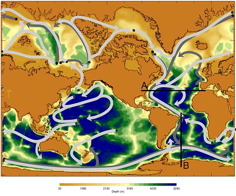
Using orthogonal curvilinear regridding of the sphere, this configuration enables a view of the role of the Arctic in global thermohaline circulation. In the figure, vectors representing the model flow have been “bundled” into flow tubes for easier visualization. A linked page describes differences between this result and a more traditional ideas. |
 |
2) extended Arctic
 |
Smaller in domain than the global view, this model setup focusses upon processes within the Arctic and their interaction with the subpolar North Atlantic. In particular this configuration allows one to study a “see-saw” as freshwater leaves the Arctic either to west or east of Greenland. This is the domain used for “CIS” study, to be described.
|
3) limited Arctic
Smaller yet, this configuration serves an efficient platform for investigating different formulations for hydro- and cryo-spheric processes within the Arctic. This has been the domain principally used for Canadian participation in “AOMIP”, to be described.
|
 |
4) Canadian Arctic Archipelago
 |
The smallest AIM domain focusses upon finer detail of ice and ocean evolution within passages in the Canadian Archipelago. Boundary conditions are supplied from the extended Arctic, itself embedded in the global domain. The figure (click to enlarge) shows flows at 22 m. |
External programs
While AIM serves research within the Institute of Ocean Sciences (IOS), it also
serves two larger programs (at this time).
1) “CIS”, Arctic ice in the 21st century
This is a collaboration led by the Canadian Ice Service (CIS) including the
Canadian Centre for Climate Analysis (CCCMA) and IOS. Modeling at CCCMA supplies
the Canadian projection for climate change until 2100. Although many features
of CCCMA projections appear quite plausible, those projections also show Arctic
ice vanishing early in the century. Such early elimination of Arctic ice may
be a model artifact. To refine projections for Arctic ice, two steps have been
taken:
a) systematic biases in CCCMA atmospheric fields were removed,
then
b) the modified (blended) fields were used to force AIM from
1950 to 2050.
The result has corrected a tendency in CCCMA to produce too little Arctic ice
during the observed period (1950-2000). Although ice volume and area are projected
to decrease during the 21st century, the ice is not expected to vanish entirely
any time early in the century.

2) “AOMIP”, international community for Arctic modeling
The Arctic Ocean Models Intercomparison Project (AOMIP) is an effort among eleven
institutions in six countries to compare different Arctic models under realistic
forcing. Canadian participation in AOMIP is from IOS utilizing AIM. Comparing
models abilities to simulate Arctic change on seasonal to decadal timescales,
AOMIP goals are to recognize differences (a) among the models and (b) from observations,
seeking to identify and correct systematic deficiencies. A link
give details of the AOMIP models and examples of intercomparison results.
Current research
1) the role of Arctic tides in global climate
Although tidal models have been run to simulate Arctic tides, models which address Arctic Ocean climate have omitted tides. If Arctic tides don’t matter to Arctic climate, surely they don’t matter to global climate. Maybe this is wrong. To a greater degree than hitherto supposed, watermass transformations that are part of global thermohaline overturning occur within the Arctic Ocean. Regions of the Arctic experience strong tidal flows, up to 3 m/s. Especially in shallow seas, such as the Barents Sea or along the Siberian shelf break, tidal dissipation yields enhanced vertical mixing, helping the Arctic lose global heat to the atmosphere and to space. Upward mixing of oceanic heat contributes also to sea ice melt. Tides have other effects on ice, creating cracks which allow ocean heat to escape and which mobilize the ice. |
 |
To explore the overlooked role of tides, AIM has expanded to include (a) botton-stress-driven
tidal mixing and (b) tidal enhancement of open water fraction in the ice cover.
2) ice and snow thickness distribution functions
 |
Sea ice is not level. It is broken by leads and crushed into pressure ridges which collide with other ridges. Blowing snow leaves drifts and bare spots.
|
3) double and differential diffusion in ocean mixing
Mixing in an ocean stratified with respect to both heat and salt can include phenomena called “salt fingers” and “layering”. Even circumstances where both heat and salt are stabilizing support “differential” mixing. A figure depicts the circum-Arctic boundary current (seen above in model flows) providing a source for long sloping intrusions into the Arctic interior. The intrusions are alternately bounded by layering and fingering. A link further describes these phenomena which are incorporated into AIM. |
 |
to Planetwater |
 |
or | more research |
 |